make_2d_arc_image

specreduce.utils.synth_data.make_2d_arc_image(nx: int = 3000, ny: int = 1000, wcs: ~astropy.wcs.wcs.WCS | None = None, extent: ~typing.Sequence[int | float] = (3500, 7000), wave_unit: ~astropy.units.core.Unit = Unit("Angstrom"), wave_air: bool = False, background: int | float = 5, line_fwhm: float = 5.0, linelists: list[str] = ['HeI'], amplitude_scale: float = 1.0, tilt_func: ~astropy.modeling.core.Model = <Legendre1D(0, c0=0.)>, add_noise: bool = True) → CCDData

Create synthetic 2D spectroscopic image of reference emission lines, e.g. a calibration arc lamp. Currently, linelists from pypeit are supported and are selected by string or list of strings that is passed to load_pypeit_calibration_lines. If a wcs is not provided, one is created using extent and wave_unit with dispersion along the X axis.

Parameters:

nxSize of image in X axis which is assumed to be the dispersion axis

nySize of image in Y axis which is assumed to be the spatial axis

wcs2D WCS to apply to the image. Must have a spectral axis defined along with

appropriate spectral wavelength units.

extentIf wcs is not provided, this defines the beginning and end wavelengths

of the dispersion axis.

wave_unitIf wcs is not provided, this defines the wavelength units of the

dispersion axis.

wave_airIf True, convert the vacuum wavelengths used by pypeit to air wavelengths.

backgroundLevel of constant background in counts

line_fwhmGaussian FWHM of the emission lines in pixels

linelistsSpecification for linelists to load from pypeit

amplitude_scaleScale factor to apply to amplitudes provided in the linelists

tilt_funcThe tilt function to apply along the cross-dispersion axis to simulate

tilted or curved emission lines.

add_noiseIf True, add Poisson noise to the image; requires photutils to be installed.

Returns:

ccd_imCCDData instance containing synthetic 2D spectroscopic image

Examples

This is an example of modeling a spectrograph whose output is curved in the cross-dispersion direction:

import matplotlib.pyplot as plt
import numpy as np
from astropy.modeling import models
import astropy.units as u
from specreduce.utils.synth_data import make_2d_arc_image

model_deg2 = models.Legendre1D(degree=2, c0=50, c1=0, c2=100)
im = make_2d_arc_image(
    linelists=['HeI', 'ArI', 'ArII'],
    line_fwhm=3,
    tilt_func=model_deg2
)
fig = plt.figure(figsize=(10, 6))
plt.imshow(im)

(Source code, png, hires.png, pdf)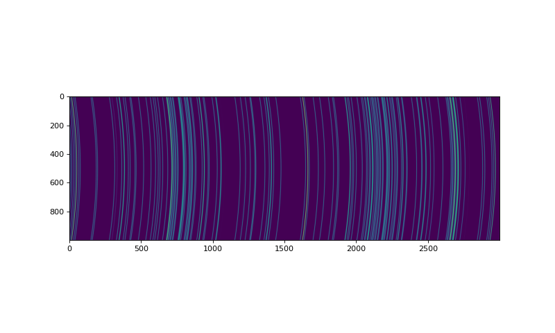

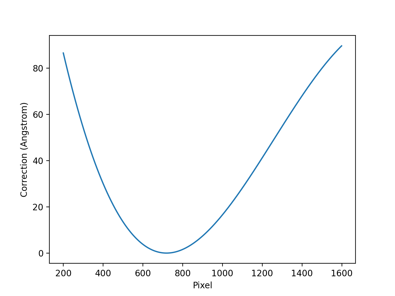
The FITS WCS standard implements ideal world coordinate functions based on the physics of simple dispersers. This is described in detail by Paper III, https://www.aanda.org/articles/aa/pdf/2006/05/aa3818-05.pdf. This can be used to model a non-linear dispersion relation based on the properties of a spectrograph. This example recreates Figure 5 in that paper using a spectrograph with a 450 lines/mm volume phase holographic grism. Standard gratings only use the first three PV terms:

import numpy as np
import matplotlib.pyplot as plt
from astropy.wcs import WCS
import astropy.units as u
from specreduce.utils.synth_data import make_2d_arc_image

non_linear_header = {
    'CTYPE1': 'AWAV-GRA',  # Grating dispersion function with air wavelengths
    'CUNIT1': 'Angstrom',  # Dispersion units
    'CRPIX1': 719.8,       # Reference pixel [pix]
    'CRVAL1': 7245.2,      # Reference value [Angstrom]
    'CDELT1': 2.956,       # Linear dispersion [Angstrom/pix]
    'PV1_0': 4.5e5,        # Grating density [1/m]
    'PV1_1': 1,            # Diffraction order
    'PV1_2': 27.0,         # Incident angle [deg]
    'PV1_3': 1.765,        # Reference refraction
    'PV1_4': -1.077e6,     # Refraction derivative [1/m]
    'CTYPE2': 'PIXEL',     # Spatial detector coordinates
    'CUNIT2': 'pix',       # Spatial units
    'CRPIX2': 1,           # Reference pixel
    'CRVAL2': 0,           # Reference value
    'CDELT2': 1            # Spatial units per pixel
}

linear_header = {
    'CTYPE1': 'AWAV',  # Grating dispersion function with air wavelengths
    'CUNIT1': 'Angstrom',  # Dispersion units
    'CRPIX1': 719.8,       # Reference pixel [pix]
    'CRVAL1': 7245.2,      # Reference value [Angstrom]
    'CDELT1': 2.956,       # Linear dispersion [Angstrom/pix]
    'CTYPE2': 'PIXEL',     # Spatial detector coordinates
    'CUNIT2': 'pix',       # Spatial units
    'CRPIX2': 1,           # Reference pixel
    'CRVAL2': 0,           # Reference value
    'CDELT2': 1            # Spatial units per pixel
}

non_linear_wcs = WCS(non_linear_header)
linear_wcs = WCS(linear_header)

# this re-creates Paper III, Figure 5
pix_array = 200 + np.arange(1400)
nlin = non_linear_wcs.spectral.pixel_to_world(pix_array)
lin = linear_wcs.spectral.pixel_to_world(pix_array)
resid = (nlin - lin).to(u.Angstrom)
plt.plot(pix_array, resid)
plt.xlabel("Pixel")
plt.ylabel("Correction (Angstrom)")
plt.show()

(Source code, png, hires.png, pdf)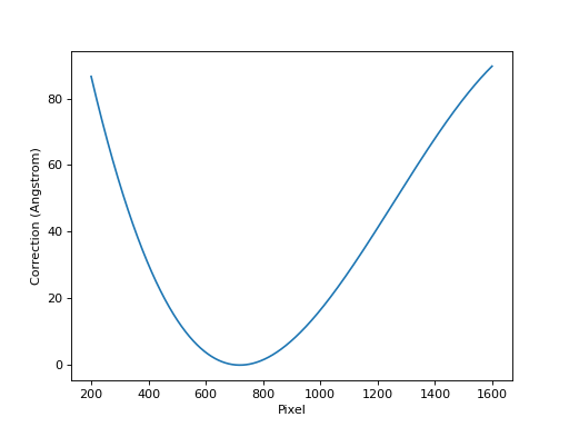

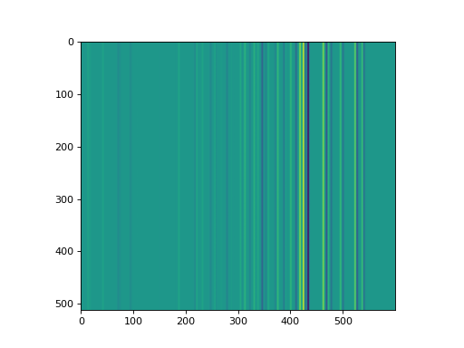
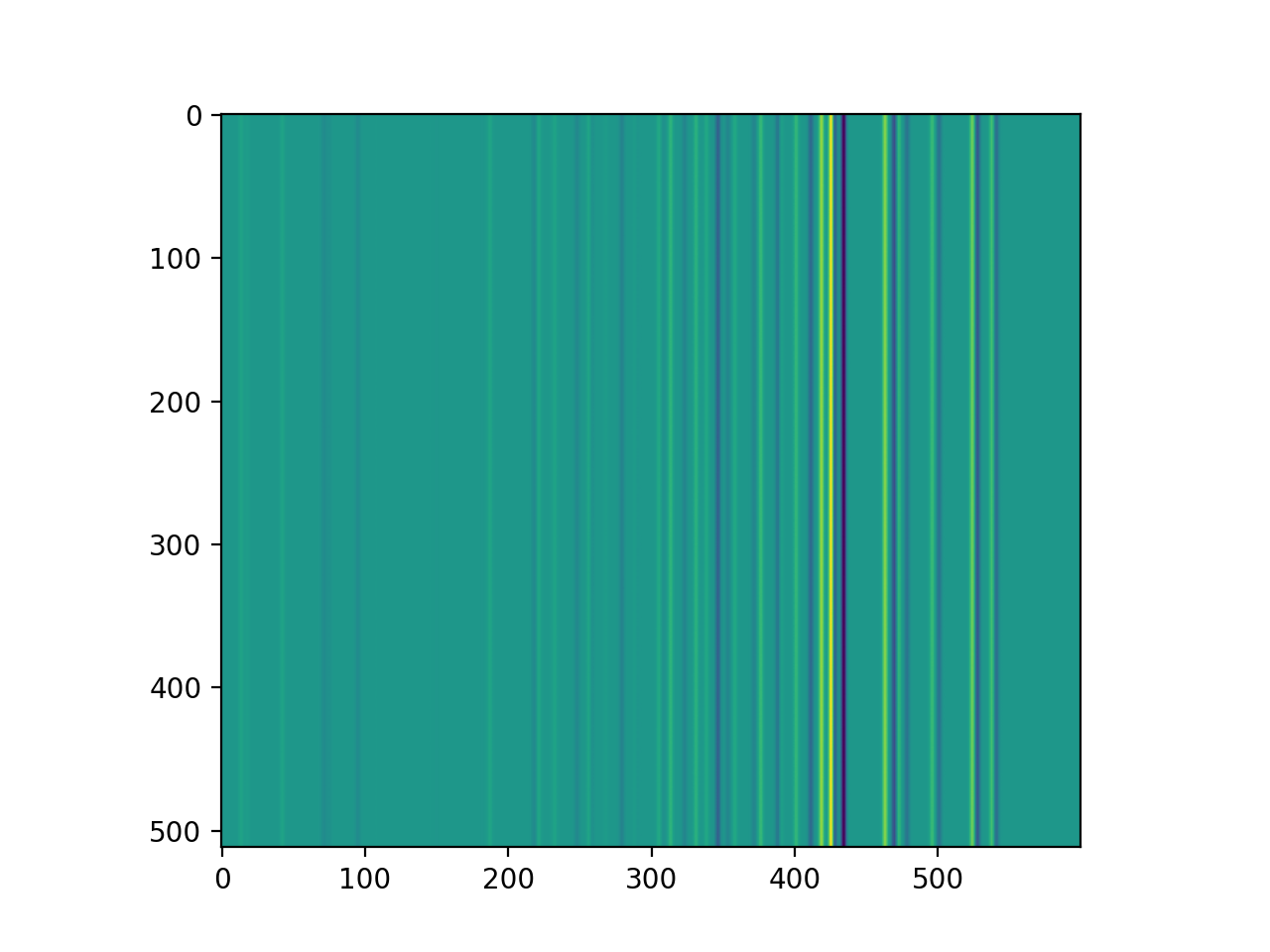
nlin_im = make_2d_arc_image(
    nx=600,
    ny=512,
    linelists=['HeI', 'NeI'],
    line_fwhm=3,
    wave_air=True,
    wcs=non_linear_wcs
)
lin_im = make_2d_arc_image(
    nx=600,
    ny=512,
    linelists=['HeI', 'NeI'],
    line_fwhm=3,
    wave_air=True,
    wcs=linear_wcs
)

# subtracting the linear simulation from the non-linear one shows how the
# positions of lines diverge between the two cases
plt.imshow(nlin_im.data - lin_im.data)
plt.show()

(png, hires.png, pdf)